PostgreSQL indexing: The basics
Posted by Simon Larsén in Programming
Back when I was in university, I had a teacher in database systems who also did contract work as a database administrator. He told me that 90% of his work was to just add and reorganize indexes to speed up queries. That was almost 10 years ago, and I'm now inclined to believe him. Having worked on three different systems backed by PostgreSQL databases over the past four years, I've seen my fair share of queries missing indexes. The fallout has ranged from a poor end user experience due to slow responses to entire systems becoming unresponsive as databases grind to a halt under the load of unindexed queries.
Needless to say, indexing is important. I would go as far as to say that if you don't understand the basics of indexing, you shouldn't be writing queries against a relational database in a production system. In this article, I'll walk you through the basics of indexing in PostgreSQL, including how an index actually works. While this is targeted at PostgreSQL and contains a lot of specifics about it, the general principles of indexing presented here are applicable to relational databases in general.
Let's get started.
Note: This article is based on PostgreSQL 16, but the vast majority of the content should be accurate for PostgreSQL 9.6 and newer.
The incredible impact of indexes
To sell you on the fact that indexes are important, let's do a quick experiment. Below I define a simple data model and fill it with some sample data.
CREATE TABLE IF NOT EXISTS data (
  id SERIAL PRIMARY KEY,
  value INT NOT NULL
);

-- seed with 10 million rows where 0 <= value <= 1,000,000
INSERT INTO data (value)
SELECT (RANDOM() * 1000000)::INT
FROM generate_series(1, 10000000);
This gives us 10 million rows, where the value is between 0 and 1 million, thus on average giving us 10 duplicates of each value. To be very clear, the data looks like this.
Note:
test=#is mypsqlprompt. I'm usingpsqlthroughout this article to execute queries.
test=# SELECT * FROM data LIMIT 5;
 id | value
----+--------
  1 | 602761
  2 | 744515
  3 | 725410
  4 | 729718
  5 | 783837
(5 rows)
Let's execute two queries, one where we search for a particular id, and one
where we search for a particular value.
test=# \timing
Timing is on.
test=# SELECT * FROM data WHERE id = 560487;
   id   | value
--------+--------
 560487 | 650515
(1 row)

Time: 0.845 ms

test=# SELECT * FROM data WHERE value = 560487;
   id    | value
---------+--------
 2068259 | 560487
 5013963 | 560487
 6894022 | 560487
 4305566 | 560487
 8455242 | 560487
 9020004 | 560487
 7313065 | 560487
(7 rows)

Time: 254.458 ms
Searching for the id took less than a millisecond, while searching for the
value took a quarter of a second. While you could argue that the database had
to do more work in compiling the results for the value search as there were
more hits, that shouldn't (and in fact, does not) account for a more than 250x
timing difference.
So what's up? Let's have a look at the query plans to find out.
test=# EXPLAIN ANALYZE SELECT * FROM data WHERE id = 560487;
                                                   QUERY PLAN
----------------------------------------------------------------------------------------------------------------
 Index Scan using data_pkey on data  (cost=0.43..8.45 rows=1 width=8) (actual time=0.016..0.017 rows=1 loops=1)
   Index Cond: (id = 560487)
 Planning Time: 0.058 ms
 Execution Time: 0.030 ms
(4 rows)

test=# EXPLAIN ANALYZE SELECT * FROM data WHERE value = 560487;
                                                     QUERY PLAN
---------------------------------------------------------------------------------------------------------------------
 Gather  (cost=1000.00..97332.43 rows=11 width=8) (actual time=74.701..257.131 rows=7 loops=1)
   Workers Planned: 2
   Workers Launched: 2
   ->  Parallel Seq Scan on data  (cost=0.00..96331.33 rows=5 width=8) (actual time=114.550..231.494 rows=2 loops=3)
         Filter: (value = 560487)
         Rows Removed by Filter: 3333331
 Planning Time: 0.046 ms
 Execution Time: 257.164 ms
(8 rows)
Going deep into query plans is beyond the scope of this article, but we don't
need to go deep here. We only need to see that the id query does an index
scan, while the value query does a seq(uential) scan. The former means that
the sought value is looked up in an index, while the latter means that the
entire table is scanned to find the value we're looking for. We can even see
that the query planner1
decided to do the sequential scan in parallel with two workers, indicating that
it's a rather heavy query.
Why was id indexed and not value, you ask? Because the primary key in a
PostgreSQL table is always indexed, but that's also the only index you get for
free. Let's now add an index to value as well and see if we can make it a bit
faster.
test=# CREATE INDEX idx_data_value ON data (value);
CREATE INDEX
test=# SELECT * FROM data WHERE value = 560487;
   id    | value
---------+--------
 2068259 | 560487
 4305566 | 560487
 5013963 | 560487
 6894022 | 560487
 7313065 | 560487
 8455242 | 560487
 9020004 | 560487
(7 rows)

Time: 1.058 ms
Look at that, as fast as searching for the id! If we have a look at the query
plan, we can see that we now do hit an index.
test=# EXPLAIN ANALYZE SELECT * FROM data WHERE value = 560487;
                                                       QUERY PLAN
------------------------------------------------------------------------------------------------------------------------
 Bitmap Heap Scan on data  (cost=4.52..48.14 rows=11 width=8) (actual time=0.050..0.072 rows=7 loops=1)
   Recheck Cond: (value = 560487)
   Heap Blocks: exact=7
   ->  Bitmap Index Scan on idx_data_value  (cost=0.00..4.52 rows=11 width=0) (actual time=0.034..0.035 rows=7 loops=1)
         Index Cond: (value = 560487)
 Planning Time: 0.189 ms
 Execution Time: 0.122 ms
(7 rows)
This looks a bit different with bitmap this and bitmap that. That's because the query planner decided that it was going to read more data, and thus opted for a slightly different strategy. We're still making good use of the index, though, and if we simply put a limit on the amount of returned values we'll see a pure index scan just like we did with the primary key.
test=# EXPLAIN ANALYZE SELECT * FROM data WHERE value = 560487 LIMIT 1;
                                                         QUERY PLAN
-----------------------------------------------------------------------------------------------------------------------------
 Limit  (cost=0.43..4.82 rows=1 width=8) (actual time=0.041..0.042 rows=1 loops=1)
   ->  Index Scan using idx_data_value on data  (cost=0.43..48.63 rows=11 width=8) (actual time=0.038..0.039 rows=1 loops=1)
         Index Cond: (value = 560487)
 Planning Time: 0.169 ms
 Execution Time: 0.077 ms
(5 rows)
If you only wanted to be sold on the fact that indexing is important, I think that's been covered already. But just having the effect of something without understanding at least the principles on which it operates will still make it harder than it has to be to apply it in practice. So let's discuss the principles of indexing and work through an example of the most commonly used index type: the B-tree.
Indexing in theory
If you've ever read a non-fiction book, you know in principle what an index is. Because at the back of that book there's a section called "index", and it contains an alphabetically sorted list of terms and phrases used throughout the book and a reference to the page number(s) where you can find their use. It's faster to find where "the rule of three" is defined in the book by looking it up in the index than by scanning through the entire book. Database indexes operate on precisely that assumption; it's faster to look a value up in an index than it is to scan through the entire table.
There are many different kinds of indexes in databases, but by far the most
common type is the B-tree index. Inspecting the indexes of the 'datatable, we
can see that they are both of typebtree`.
test=# \d data
                            Table "public.data"
 Column |  Type   | Collation | Nullable |             Default
--------+---------+-----------+----------+----------------------------------
 id     | integer |           | not null | nextval('data_id_seq'::regclass)
 value  | integer |           | not null |
Indexes:
    "data_pkey" PRIMARY KEY, btree (id)
    "idx_data_value" btree (value)
You may immediately think "oh, a binary tree", which is close, but no cigar. In the following section I'll outline how a B-tree index works and its properties such that you can make effective use of it in your day to day work.
The B-tree
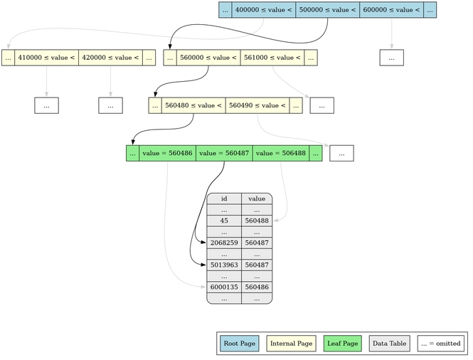
A B-tree is indeed a search tree, and it is in fact rather similar to a binary search tree. Each node, or page2 is a sorted list of references either to other pages of the tree, or to columns of the indexed table3
Let's work through the example of searching for value=560487 given the index
structure shown in the image below. We start from the root page and search
4
through it until we find the segment where 500000 <= value. Semantically, this
segment has an exclusive upper limit equal to the inclusive lower limit of the
next segment (i.e. 500000 <= value < 600000 in this example). Following the
reference to the start of the next page, we search that until we find the
segment where 560000 <= value < 561000. This segment refers to a leaf page,
which again we search through until we find the desired key that in turn
contains references to the sought rows of the table. This search path is
reflected in the below image with black lines, whereas the faint gray lines
show existing references that are not traversed.

Note that this is just for illustrative purposes. The splitting into segments as shown here is completely made up by me to be easy to illustrate. It's very unlikely to actually be a good split and therefore not the one that PostgreSQL would actually make.
In addition to providing quick lookup to specific values, the fact that B-trees are sorted leads to some possibly unexpected benefits in queries that require sorted output.
Selecting ranges is almost as fast as single values
Did you notice in the illustration above that the leaf page contained not only the value we searched for, but also its closest neighbors? Because of this adjacency, an index lookup for a range of values is incredibly efficient5.
test=# SELECT * FROM data WHERE 560486 <= value AND value < 560489;
   id    | value
---------+--------
 1061367 | 560488
 1451289 | 560488
 2068259 | 560487
 2250572 | 560488
 2298922 | 560486
 2998709 | 560486
 3149734 | 560486
 3385911 | 560486
 3552143 | 560488
 4123068 | 560488
 4305566 | 560487
 4599351 | 560488
 5013963 | 560487
 5490314 | 560488
 5521774 | 560488
 5715474 | 560486
 5725443 | 560488
 6125940 | 560486
 6423931 | 560486
 6752395 | 560488
 6894022 | 560487
 7313065 | 560487
 7365878 | 560488
 7956607 | 560488
 8046840 | 560486
 8290267 | 560488
 8455242 | 560487
 8941102 | 560488
 9020004 | 560487
 9663961 | 560488
(30 rows)

Time: 1.360 ms
A very common use case for a range selection is on creation date, e.g. `WHERE created_at >= '2024-04-01'.
Indexes greatly speed up ORDER BY
Tacking on an ORDER BY to a query is commonplace and pretty much required if
you plan to do any kind of pagination on the result set6. Without an index on value, ordering by it takes quite a bit of
time.
test=# DROP INDEX IF EXISTS idx_data_value;
DROP INDEX
test=# SELECT * FROM DATA ORDER BY value LIMIT 10;
   id    | value
---------+-------
 1453865 |     0
 8150282 |     0
 7796750 |     0
 3782708 |     0
 8571152 |     1
 1650656 |     1
 9165134 |     1
  268472 |     1
 5889252 |     1
 3330397 |     1
(10 rows)

Time: 331.239 ms
But tacking on the index, it's again orders of magnitude faster.
test=# CREATE INDEX idx_data_value ON data (value);
CREATE INDEX
test=# SELECT * FROM DATA ORDER BY value LIMIT 10;
   id    | value
---------+-------
 1453865 |     0
 3782708 |     0
 7796750 |     0
 8150282 |     0
  268472 |     1
 1650656 |     1
 2191333 |     1
 3330397 |     1
 5364764 |     1
 5889252 |     1
(10 rows)

Time: 1.628 ms
This is so fast because there's actually no ordering going on; PostgreSQL just scans the already sorted index.
test=# EXPLAIN ANALYZE SELECT * FROM DATA ORDER BY value LIMIT 10;
                                                               QUERY PLAN
----------------------------------------------------------------------------------------------------------------------------------------
 Limit  (cost=0.43..0.81 rows=10 width=8) (actual time=0.049..0.074 rows=10 loops=1)
   ->  Index Scan using idx_data_value on data  (cost=0.43..372326.50 rows=10000000 width=8) (actual time=0.046..0.069 rows=10 loops=1)
 Planning Time: 0.161 ms
 Execution Time: 0.104 ms
(4 rows)

Time: 1.284 ms
There is simply a lot of value to having an index that is already ordered7 as so many common operations rely on ordering.
Indexing pitfalls
Thus far, this article has mostly covered the happy path of indexing, when everything just works out. It may have given you the impression that indexing is a silver bullet to any query running a bit slow. Unfortunately, that's far from the case, so in this section I will outline a few scenarios that may cause confusion among up and coming indexers.
The query planner can choose not to use an index
Indexes are great, but sometimes the query planner may choose to ignore them and
just scan the table instead. This is quite easy to show, take for example the
following query where we search for any value > 500000.
test=# EXPLAIN ANALYZE SELECT * FROM data WHERE value > 500000;
                                                   QUERY PLAN
-----------------------------------------------------------------------------------------------------------------
 Seq Scan on data  (cost=0.00..169248.00 rows=5044664 width=8) (actual time=5.213..653.177 rows=4998152 loops=1)
   Filter: (value > 500000)
   Rows Removed by Filter: 5001848
 Planning Time: 0.151 ms
 JIT:
   Functions: 2
   Options: Inlining false, Optimization false, Expressions true, Deforming true
   Timing: Generation 0.379 ms, Inlining 0.000 ms, Optimization 0.356 ms, Emission 3.469 ms, Total 4.204 ms
 Execution Time: 770.366 ms
(9 rows)
The query planner chooses to forego the index and just scan the table (Seq Scan
on data). Why? Recall again the example trace of the B-tree index in the first
section of this article; it requires resolving a whole bunch of references and
accessing data both from the index and the table8,
which are stored separately. When accessing large parts of the table, it's often
faster to just scan through the entire table than it is to resolve all of those
references. The condition value > 500000 corresponds to roughly half of the
table9,
so the query planner does not use the index.
If we increase the value, the query planner will re-evaluate and use the index as it estimates that a small enough part of the table needs to be scanned in the end.
 Bitmap Heap Scan on data  (cost=49658.83..144439.73 rows=4042632 width=8) (actual time=196.822..663.746 rows=4000401 loops=1)
   Recheck Cond: (value > 600000)
   Heap Blocks: exact=44248
   ->  Bitmap Index Scan on idx_data_value  (cost=0.00..48648.17 rows=4042632 width=0) (actual time=189.479..189.479 rows=4000401 loops=1)
         Index Cond: (value > 600000)
 Planning Time: 0.157 ms
 JIT:
   Functions: 2
   Options: Inlining false, Optimization false, Expressions true, Deforming true
   Timing: Generation 0.367 ms, Inlining 0.000 ms, Optimization 0.000 ms, Emission 0.000 ms, Total 0.367 ms
 Execution Time: 756.080 ms
(11 rows)
Now the index is used, but the query runs almost precisely as fast at 756 ms,
compared to 770 ms for the full table scan. Considering it's also fetching
fewer rows due to a narrower search, the fact that the query planner chose to
run the previous plan without touching the index seems justified.
Note that this is all circumstantial, and that's entirely the point. The query planner will come up with different query plans depending on the layout of the data and the exact parameters of the query, even with all other server and client settings being the same. A consequence of this is query plans can change dramatically as data in your tables accumulate. This also means that the query plans you get in your local development environment are often different from the ones you get in production. As such, one can easily be fooled by a query that gets a terrible looking plan in your local environment but actually runs fine in production, and vice versa10. Be aware of this when you add new indexes and are perplexed as to why they are not used; there may just not be enough data for it to be worth it.
An index is for an exact expression
We have an index on data(value) and showed that ordering by value is super
quick. Let's do it again so you don't have to scroll up too far.
test=# SELECT * FROM data ORDER BY value LIMIT 10;
   id    | value
---------+-------
 1453865 |     0
 3782708 |     0
 7796750 |     0
 8150282 |     0
  268472 |     1
 1650656 |     1
 2191333 |     1
 3330397 |     1
 5364764 |     1
 5889252 |     1
(10 rows)

Time: 0.455 ms
But what if we order by value * 2?
test=# SELECT * FROM data ORDER BY value * 2 LIMIT 10;
   id    | value
---------+-------
 3782708 |     0
 1453865 |     0
 7796750 |     0
 8150282 |     0
 5889252 |     1
 3330397 |     1
 9165134 |     1
 5364764 |     1
 8571152 |     1
  268472 |     1
(10 rows)

Time: 540.665 ms
It takes 1000 times as long. Looking at the query plan, we can see why.
test=# EXPLAIN ANALYZE SELECT * FROM data ORDER BY value * 2 LIMIT 10;
                                                                 QUERY PLAN
--------------------------------------------------------------------------------------------------------------------------------------------
 Limit  (cost=187371.53..187372.70 rows=10 width=12) (actual time=691.290..696.029 rows=10 loops=1)
   ->  Gather Merge  (cost=187371.53..1159661.72 rows=8333334 width=12) (actual time=682.579..687.316 rows=10 loops=1)
         Workers Planned: 2
         Workers Launched: 2
         ->  Sort  (cost=186371.51..196788.18 rows=4166667 width=12) (actual time=659.729..659.730 rows=7 loops=3)
               Sort Key: ((value * 2))
               Sort Method: top-N heapsort  Memory: 25kB
               Worker 0:  Sort Method: top-N heapsort  Memory: 25kB
               Worker 1:  Sort Method: top-N heapsort  Memory: 25kB
               ->  Parallel Seq Scan on data  (cost=0.00..96331.33 rows=4166667 width=12) (actual time=1.799..312.822 rows=3333333 loops=3)
 Planning Time: 0.250 ms
 JIT:
   Functions: 7
   Options: Inlining false, Optimization false, Expressions true, Deforming true
   Timing: Generation 1.026 ms, Inlining 0.000 ms, Optimization 0.738 ms, Emission 13.207 ms, Total 14.971 ms
 Execution Time: 696.794 ms
(16 rows)
Again, there is no need for a deep understanding of query plans to see that this
is worse than the simple index scan shown before. Here we've both got sequential
scanning of the entire table and a bunch of sorting going on, ending up taking a
whole lot of time. The reason the query plan looks like that is that value * 2
is not indexed, only value is. It's the exact expression used in the index
creation that is actually indexed and can be used in WHERE, ORDER BY, GROUP
BY etc. This should be fairly evident given how a B-tree index lookup works; we
cannot quickly lookup an arbitrary expression using a column based on an index
of the raw column.
This example is of course silly, because ordering by a value or ordering by
double that value results in the same order. In a more realistic scenario, there
are many good reasons to use expressions in ordering or searching. For example,
if you want to perform a case insensitive search on a text column that contains
mixed casing, calling LOWER() on that column makes a whole lot of sense. Such
searches can be optimized using an expression index (a.k.a functional
index), but
that is something I plan to cover in an upcoming article. For the purposes of
this article, I only want to make it very clear that a column having an index on
it does not imply that any search on that column can utilize said index.
Indexes optimize reads but slow down writes
Something to keep in mind with indexing is that an index is made to speed up reads. On the flip side, they slow down writes as every time a table is written to its indexes must also be written to11
That said, you probably don't need to worry much about indexes taking up space or slowing down writes. I have personally only had to think about such things with indexes for very large tables with billions of rows, or tables with very high throughput demands. The vast majority of applications have neither of those, while the lack of indexes becomes problematic even for small amounts of data. In other words, the benefits of indexing almost always outweighs the cons, but it's good to be aware that cons exist.
Summary
In this article, we've covered the basics of indexing in PostgreSQL, had a theoretical look at a B-tree index and its properties as well as how these can be taken advantage of. In addition, we've looked at some common pitfalls with indexing and some things to keep in mind. That may seem like a lot more than just basics, but the unfortunate reality is that indexing is a complex subject. We haven't delved into other types of indexes or multicolumn indexes. We also haven't touched upon partial indexes or how indexes interact with more complex queries, such as joins. Simply put, there is a lot more to cover.
I plan to continue this article series with shorter articles that cover specific use cases where these more advanced indexing techniques are useful. If you're eager to learn more before I get around to that, the PostgreSQL index documentation is a great place to start!
- The query planner (or optimizer) is the part of PostgreSQL that's responsible for taking your high-level SQL query and figuring out the fastest way to execute it in the database (source). ↩
- In PostgreSQL, the nodes of a B-tree are called pages (source) ↩
- Pages in the B-tree are either internal pages or leaf pages. An internal page only contains references to other B-tree pages, while a leaf page only contains references to the indexed table. There are no hybrid internal/leaf pages. The root can be either internal or a leaf depending on the size of the index. There is also a special metapage that keeps track of things like tree depth and which page is the root of the tree (source). A search in a B-tree index starts from the singular root page and then proceeds through internal pages in the tree until a leaf page containing references to the indexed table is found. From there, the references to the table can be resolved and the rows retrieved. ↩
- The page is sorted, PostgreSQL makes effective use of binary search to quickly find a key ↩
- Depending on the amount of hits, scanning the rows from the table may of course take longer, however. ↩
- The order in which
rows are returned from a query is undefined unless
ORDER BYis provided. A common bug in backend systems is thatOFFSETandLIMITare used for pagination either without explicit ordering or with ordering that is not unique. ↩ - Note that only the B-tree type of index has this property (source). ↩
- Except for so-called index-only scans (source) ↩
- The query planner knows this as PostgreSQL keeps statistics on table contents (source). ↩
- The query planner can also come up with terrible queries if table statistics are too outdated, but that's a topic for another time. ↩
- Except for heap-only tuples (source). Indexes can also take up a significant amount of storage. I once worked with a production database where the largest table was around 2 terabytes in size, with an additional 3 terabytes of indexes. Adding a new index was something we thought long and hard about before actually doing. ↩